A. K. BEETLE

Lets briefly explore the fundamental concepts of deep learning algorithms.

1.   ATTENTION MECHANISMS

Attention mechanisms enhance performance by enabling models to assign dynamic importance (weights) to different input features, helping to prioritize different aspects of the training data.

The core idea is to compute the similarity between the query (what we are looking for) and the key (descriptor of available information), which is then used to decide how much of each value (content to be retrieved) we need to focus on.

The most common mathematical operation performed is a scaled dot-product attention computation done in three sequential steps:

• Determine the dot product between queries and keys.
• Apply a softmax activation to turn them into attention weights.
• Use these weights to compute a weighted sum of the values.

Some commonly used attention mechanisms include:

(1) Soft Attention: Continuous, differentiable and used in training deep networks.

(2) Hard Attention: Makes discrete choices on which inputs to attend to and is non-differentiable in nature. Useful for reinforcement learning.

(3) Self-Attention: Helps in modeling sequences and is the backbone of Transformer architectures. Each element in the sequence attends to all other elements.

(4) Cross-Attention: During tasks such as machine translation (aligning source and target sentences), it lets the queries come from one sequence and keys/values from another.

A more effective attention mechanism is Multi-Head Attention that run several operations in parallel (each learning different representations such as short-range dependencies or long-range context for example). The outputs are eventually concatenated and linearly transformed to combine perspectives.

2.   ACTIVATION FUNCTIONS

Activation functions introduce non-linearity into the neural network, allowing it to learn complex relationships between inputs and outputs.

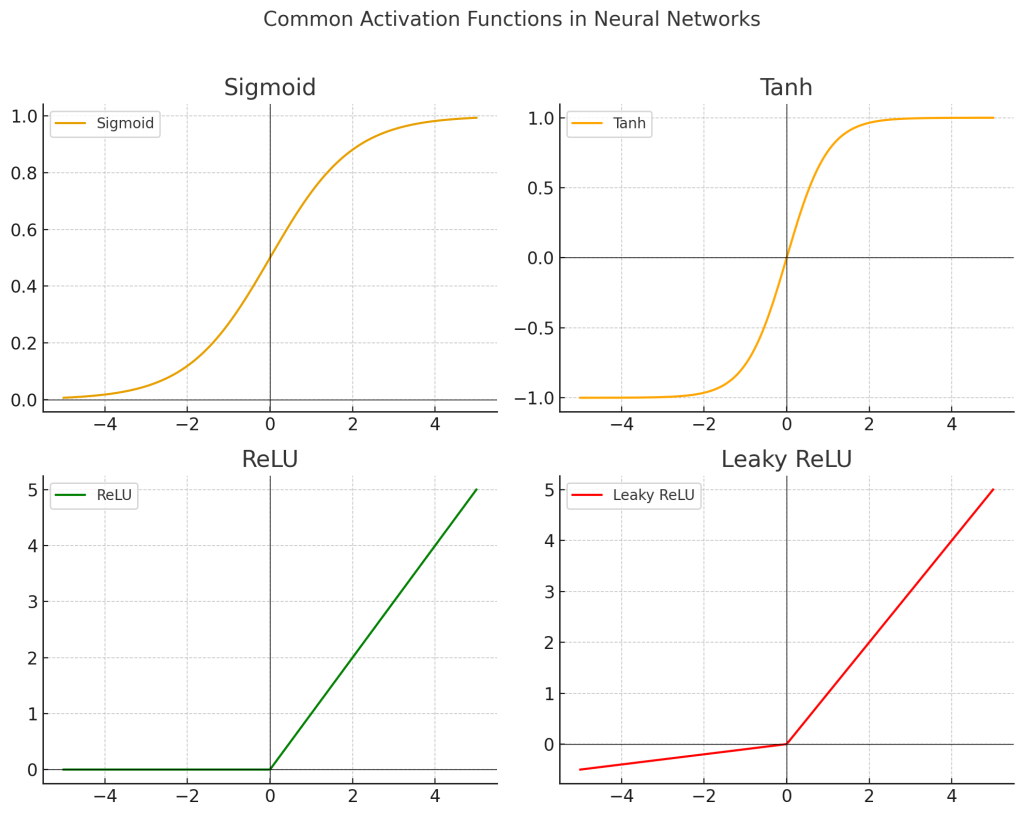
Common activation functions include:

– Sigmoid: Compresses inputs to the range (0, 1) and useful for binary classification, but suffers from vanishing gradients (gradients shrink for very large and very small inputs) that can slow down learning.

– Tanh (Hyperbolic Tangent): Ranges from (-1, 1), with improved gradient behavior over sigmoid (zero-centering helps optimization).

– ReLU (Rectified Linear Unit): Outputs the input directly if positive; otherwise, outputs zero. It’s computationally efficient and helps mitigate the vanishing gradient problem. However, in certain cases some neurons can output zero for all inputs and stop learning (dying ReLU problem).

– Softplus: A smooth and continuous approximation of ReLU. It softens the hard, non-differentiable transition of ReLU at zero.

– Leaky ReLU: Allows a small gradient when the unit is not active, to avoid dead neurons.

– Sigmoid Linear Unit (SiLU or Swish): Smooth and self-gated, often outperforms ReLU in deeper networks.

– Exponential Linear Unit (ELU): Produces negative outputs to push mean activations closer to zero.

– Softmax: Used in output layer for multi-class classification and converts an vector of raw scores into probabilities.

3.   WEIGHT OPTIMIZATION

Training a neural network involves optimizing its weights to minimize prediction error, as computed by a loss function. This is typically done using a gradient-based optimization algorithm, most commonly gradient descent.

Gradient is the change in loss with change in weights. Weights are the parameters that connect the neurons in a neural weight and they store the ‘knowledge‘ that the neural net learns during training. Initially, they are set randomly and the network optimizes these weights iteratively during the training process.

The gradients represent the sensitivity of the loss (calculated by the loss function) with respect to each weight. Backpropagation (backward propagation of the errors by applying the chain rule of differential calculus) is an algorithm usually used to calculate the gradients after each forward pass of input data and subsequent loss calculation. The gradients are then used by the optimizers to update the weights towards a minima.

Optimization Techniques:

– Batch Gradient Descent: Computes gradients over the entire training set but is computationally intensive and may converge slowly.
– Mini-Batch Gradient Descent: Updates weights using small subsets (mini-batches) of the training data. This is a balance between batch and stochastic gradient descent, offering stability and efficiency.
– Stochastic Gradient Descent (SGD): Updates weights per instance—fast but noisy.

To further enhance the training process, the following concepts are often used:

(1) Learning Rate: The learning rate is a hyperparameter that determines to what extent the new weights overrides the older weights. The learning rate (varying between 0 and 1) needs to be adjusted during training based on past gradients (a low value implies long training time and a high value implies exploding loss).

(2) Momentum: Accelerates convergence by dampening oscillations and is used to decide the weights based on previous weights (adaptively changing the step size).

(3) Early Stopping: The error on a validation set is monitored so as to end the training when the loss does not change. And the necessary details are saved to reuse the model.

4.   LOSS FUNCTIONS

Loss functions quantify the difference between predicted and true values. They provide tools for precise measurement of the prediction error that help in monitoring the performance of weight optimization algorithms.

Different tasks require different types of loss functions and the choice affects both the training and the final performance of of a neural net.

1. For Classification:

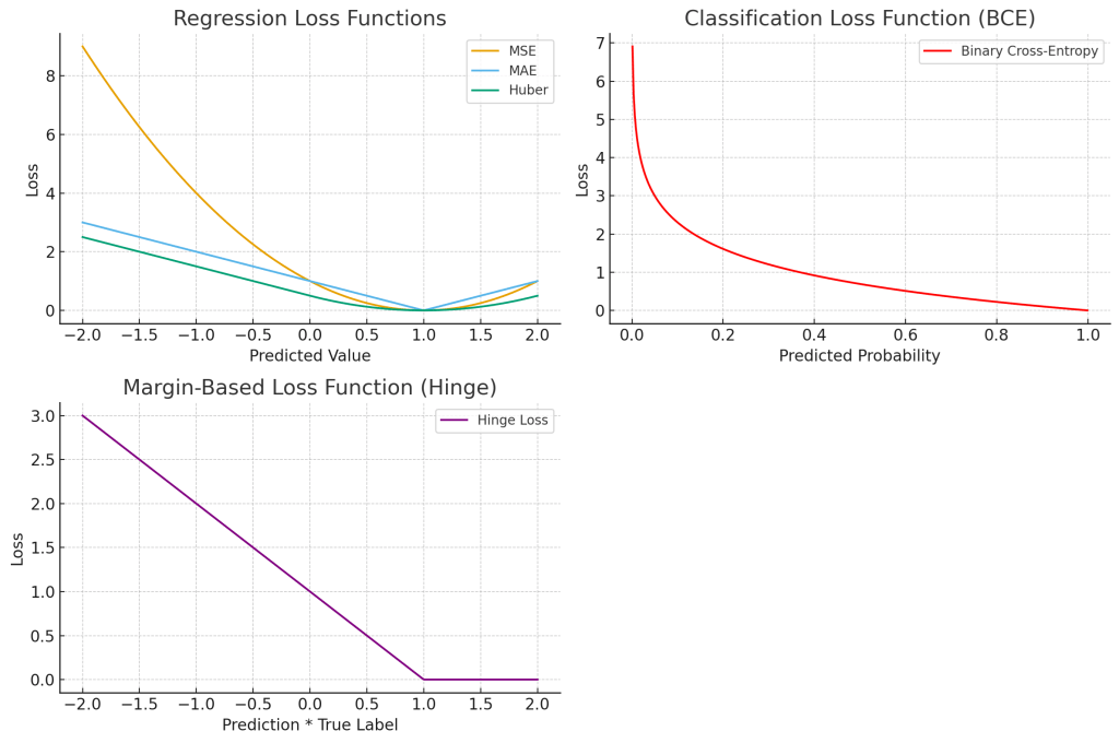
– Cross-Entropy Loss (Log Loss): Measures the performance of classification models whose output is a probability distribution.

– Kullback-Leibler Divergence (Relative Entropy): Measures the statistical differential between a predicted probability distribution and a reference probability distribution. The baseline may be a training production window or a validation dataset. This loss function is useful for variational autoencoders.

2. For Regression:

– Mean Squared Error (MSE): Penalizes larger errors more heavily, but useful for smooth regression tasks.
– Mean Absolute Error (MAE): More robust to outliers than MSE.

3. For Relative Ordering:

– Hinge Loss: Useful for classification with margins.

– Contrastive Loss: Common in Siamese nets, it helps to keep similar embeddings close and dissimilar ones far apart.

NOTES:

– Special loss functions that are used at times are Dice Loss (for image segmentation masks), Perpetual Loss (in style transfer and super-resolution) and Custom Loss (finance, healthcare, reinforcement learning, etc.).

– An effective loss function needs to be mathematically differentiable, sensitive and aligned with the goal of the task in hand.

5.   REGULARIZATION METHODS

Regularization techniques are essential to prevent overfitting and improve the generalization ability of neural networks. It is a set of strategies to constrain the neural net from learning and overfit noisy training data.

Popular methods include:

(1) Dropout: Randomly deactivates a subset of neurons (set to zero) during training, controlled by a dropout rate hyperparameter. This prevents the network from becoming too reliant on specific neurons. However, during testing all neurons are used (but with scaled outputs to account for the training).

(2) Weight Penalties (L1 & L2 Regularizations): Adds a penalty term to the loss function for large weights. L1 promotes interpretability and feature selection and L2 helps in improving stability.

(3) Batch Normalization (Indirect Regularization): Normalizes intermediate layer outputs across mini-batches to stabilize and accelerate training. Batches help in reducing sensitivity to weight initialization and can lower the need for dropouts.

(4) Layer Normalization: Normalizes within each data samples across features rather than batches—particularly useful in sequence models and attention-based architectures (like Transformers).

Note – Advanced regularization methods include weight sharing filters (in CNNs), adversarial training, label smoothening, etc.

Having explored the mathematical basis of neural nets, let us now move on to understanding some of the most common neural networks in use today.